
Factor analysis can be conducted in different ways. A common approach is linear regression using a simple model like Ordinary Least Squares (OLS). While we believe this is a good starting point, using solely OLS can have drawbacks.
This case study demonstrates how a two-step approach, using a Lasso regression for initial factor selection followed by an OLS regression for factor exposures and significance among the selected factors, can enhance the interpretability and accuracy of factor analysis.
At its core, Venn is a factor-based tool, as many of its features are powered by analysis using the Two Sigma Factor Lens. Factor analysis can be conducted in different ways. One common method is linear regression, which is a technique that uses explanatory variables (factors, in our case) to model a dependent variable (portfolio or investment returns, in our case). The simple regression model that is typically covered in Statistics 101 courses is Ordinary Least Squares (OLS), which seeks to minimize the sum of the squares of the differences between the dependent variable and those predicted by the model of explanatory variables. OLS is a good starting point for factor analysis, however we believe using solely OLS can have drawbacks.
We believe a two-step approach can enhance the interpretability and accuracy of factor analysis:
- Lasso regression: A factor selection technique that seeks to reduce the full set of factors in the Two Sigma Factor Lens to those the lasso regression determines to be most relevant to each portfolio’s or investment’s returns
- OLS regression: A standard regression that seeks to explain the portfolio’s or investment’s returns using the selected factors from step 1
Why is the first step necessary? While OLS regressions are computationally simple and typically well-behaved, a key drawback is that they attempt to fit every possible explanatory factor to the dependent variable, even if the relationship is rather weak. We’ll illustrate this through a simple case study. Here is the set up:
- We constructed 7 explanatory factors of 36 data points each. The factors are completely random values within a normal distribution with a mean of zero and a standard deviation of 2%.
- We constructed a “noise” data stream that also has 36 data points with random values pulled from a normal distribution with a mean of zero and a standard deviation of 0.5%.
- We constructed a dependent return stream using 100% of Factor 1 + 50% of Factor 2 + 30% of Factor 3 + “noise” data. The dependent return stream has no relationship to Factors 4 through 7.
Simply running an OLS regression to fit the dependent return stream to the 7 random factors yields the results in Exhibit 1:
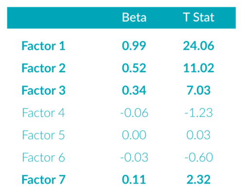
Exhibit 1: OLS Regression
As expected, the betas to Factors 1 through 3 are close to the original values used to construct the dependent return stream. They are also statistically significant, as demonstrated by the t-statistic values. These values measure how confident we are in the beta estimates. T-statistics greater than an absolute value of approximately 2.00 tell us that we are 95% confident that the factor’s beta is statistically different from zero.
However, the regression also identified betas to all of the factors, and even found a 0.11 relationship to Factor 7 to be statistically significant, even though we know there is no ex-ante relationship.
Lasso regressions1 can be used to select a subset of factors that appear to provide the greatest explanatory power. Here are the results of a lasso regression using the dependent variable and the 7 random factors:

Exhibit 2: Selected Factors from Lasso Regression
The lasso regression filtered out those factors that had no ex-ante relationship with the dependent variable.
Finally, we will run an OLS regression using only those explanatory variables selected by the lasso regression. The results are displayed in Exhibit 3:
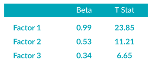
Exhibit 3: OLS Regression with Lasso Regression Selected Factors
Again, as expected, the betas to Factors 1 through 3 are very close to the original values used to construct the dependent return stream. While the t-statistics for the factors differ marginally from Exhibit 1, the important point is that they are still statistically significant.
We believe the results of this regression are simpler and easier to interpret. Additionally, the process of selecting more relevant and intuitive factors may help improve the interpretation of the inherent risk drivers as well as enhance the accuracy of the analysis by discarding the noise of irrelevant factors.
References
1 Additional reading on lasso regressions:
Cavanaugh, J. E. (1997). “Unifying the derivations of the Akaike and corrected Akaike information criteria”, Statistics & Probability Letters, Vol. 33, No. 2, pages 201-208.
Efron, B., Johnstone, I., Hastie, T. and Tibshirani, R. (2002). Least angle regression. Annals of Statistics, Vol. 32, No. 2, pages 407-499.
Tibshirani, R. (1996). Regression shrinkage and selection via the lasso. J. Royal. Statist. Soc B., Vol. 58, No. 1, pages 267-288.
This article is not an endorsement by Two Sigma Investor Solutions, LP or any of its affiliates (collectively, “Two Sigma”) of the topics discussed. The views expressed above reflect those of the authors and are not necessarily the views of Two Sigma. This article (i) is only for informational and educational purposes, (ii) is not intended to provide, and should not be relied upon, for investment, accounting, legal or tax advice, and (iii) is not a recommendation as to any portfolio, allocation, strategy or investment. This article is not an offer to sell or the solicitation of an offer to buy any securities or other instruments. This article is current as of the date of issuance (or any earlier date as referenced herein) and is subject to change without notice. The analytics or other services available on Venn change frequently and the content of this article should be expected to become outdated and less accurate over time. Any statements regarding planned or future development efforts for our existing or new products or services are not intended to be a promise or guarantee of future availability of products, services, or features. Such statements merely reflect our current plans. They are not intended to indicate when or how particular features will be offered or at what price. These planned or future development efforts may change without notice. Two Sigma has no obligation to update the article nor does Two Sigma make any express or implied warranties or representations as to its completeness or accuracy. This material uses some trademarks owned by entities other than Two Sigma purely for identification and comment as fair nominative use. That use does not imply any association with or endorsement of the other company by Two Sigma, or vice versa. See the end of the document for other important disclaimers and disclosures. Click here for other important disclaimers and disclosures.
This article may include discussion of investing in virtual currencies. You should be aware that virtual currencies can have unique characteristics from other securities, securities transactions and financial transactions. Virtual currencies prices may be volatile, they may be difficult to price and their liquidity may be dispersed. Virtual currencies may be subject to certain cybersecurity and technology risks. Various intermediaries in the virtual currency markets may be unregulated, and the general regulatory landscape for virtual currencies is uncertain. The identity of virtual currency market participants may be opaque, which may increase the risk of market manipulation and fraud. Fees involved in trading virtual currencies may vary.